
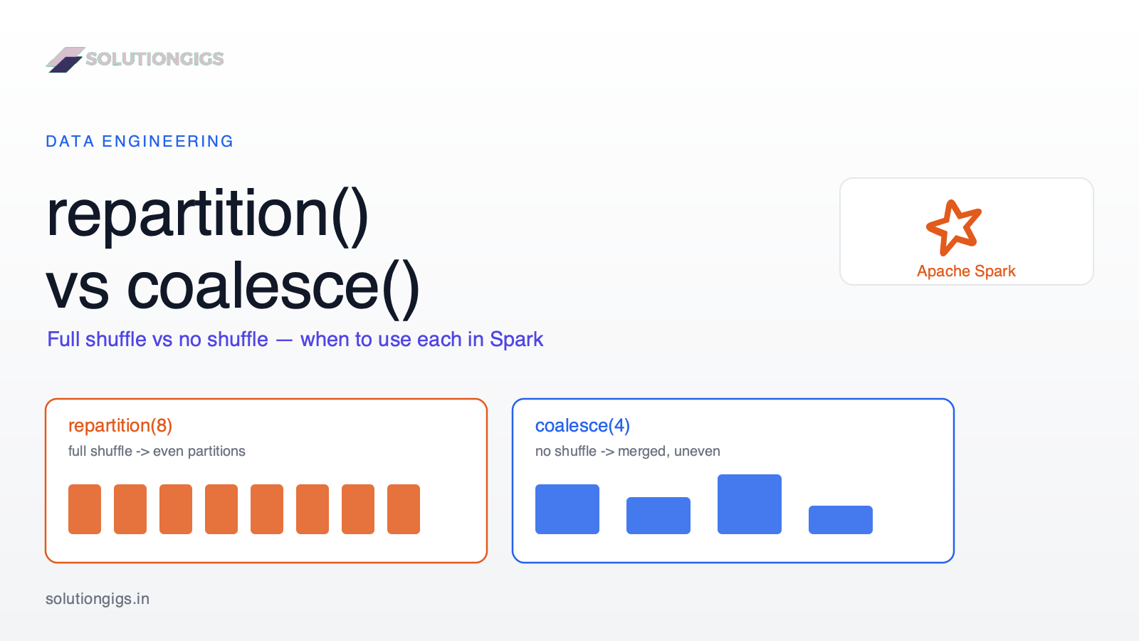
Spark repartition() vs coalesce(): When to Use Each
Last Updated: July 2026 | 14 min read
Quick Answer: In Apache Spark, repartition() does a full shuffle to redistribute rows evenly across a target number of partitions, and can both increase and decrease the count. coalesce() avoids a full shuffle by merging existing partitions on the same executors — so it's far cheaper, but it can only decrease the count and may leave partitions unevenly sized. Rule of thumb: shrinking partitions after a heavy filter, right before a write → coalesce(); increasing partitions, fixing skew, or partitioning by a column → repartition(). The classic trap is coalesce(1), which collapses parallelism across the entire upstream computation, not just the write.
repartition() vs coalesce() is one of the most-asked Spark questions — in interviews and in real 2 a.m. debugging sessions — and the usual one-liner ("coalesce is cheaper") hides the detail that actually bites you in production. Both change how many partitions your data lives in, but how they do it is completely different, and picking the wrong one either wastes a full shuffle or silently throttles your whole job to a single core. This guide explains exactly what each does under the hood, gives you a decision rule you can apply without thinking, and walks through the real PySpark patterns — including the coalesce(1) trap that catches almost everyone once.
The core difference: it's all about the shuffle
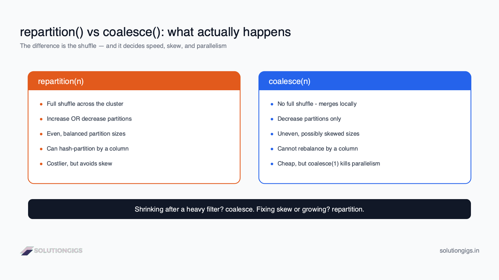
repartition() triggers a full shuffle to produce evenly-sized partitions; coalesce() skips the shuffle by merging partitions locally, which is cheaper but can leave sizes unbalanced. That single distinction — shuffle or no shuffle — drives every other trade-off between them.
A partition is the unit of parallelism in Spark: one partition is processed by one task on one core. A shuffle is the expensive operation of moving data across the network between executors so it can be regrouped. Shuffles are the most costly thing Spark does — they write to disk, serialize data, and cross the network — so avoiding an unnecessary one is a real win, and forcing one you don't need is a real waste.
repartition(n)hash-partitions or round-robin distributes every row acrossnnew partitions. Every row potentially moves. The payoff: partitions come out balanced and evenly sized.coalesce(n)merges existing partitions intonwithout moving data across the network where it can avoid it. Executors keep their local partitions and just combine them. The catch: if partition sizes were uneven to begin with, the merged result is uneven too.
Mental model:
repartition()is reshuffle the whole deck and deal evenly.coalesce()is stack a few piles together without redealing. One is fair but slow; the other is fast but lumpy.
repartition(): full shuffle, even distribution, any direction
repartition(n) always shuffles, always produces balanced partitions, and can move the count up or down. Use it when you need even distribution or more partitions than you have now.
# Increase partitions — only repartition can do this
df_more = df.repartition(200)

# Decrease with even sizing (e.g. after skew) — pays a shuffle for balance
df_even = df.repartition(50)

# Repartition by a column — co-locate rows with the same key
df_keyed = df.repartition("customer_id")

# By count AND column
df_keyed_n = df.repartition(100, "customer_id")
Because it shuffles, repartition() is the tool for three jobs coalesce() simply cannot do:
- Increasing the partition count — e.g. reading a few large files but wanting more parallelism.
- Rebalancing skew — if one partition holds 90% of the rows, a shuffle spreads them out. This is a first-line fix for Spark data skew.
- Partitioning by a column — hash-partition on a join or group key so matching rows are co-located, cutting the shuffle in the next stage.
repartition(col) vs partitionBy() — don't confuse them
These sound alike but act on different layers:
df.repartition("date")controls the in-memory partition distribution (how many tasks, which rows together).df.write.partitionBy("date")controls the on-disk directory layout (/date=2026-07-24/...).
A common high-performance write pattern combines both — repartition("date") so each date's rows are in one partition, then partitionBy("date") on the writer — which produces one clean file per date instead of hundreds of tiny fragments. That directly attacks the Spark small files problem; the trade-offs of on-disk layout are covered in the data partitioning strategies guide.
coalesce(): no shuffle, decrease only, watch the skew
coalesce(n) reduces the partition count by merging partitions locally without a full shuffle, making it the cheap choice for shrinking — but it can only go down, and the merged partitions may be uneven. It's the right tool immediately before writing output that's been thinned out.
# Heavy filter leaves 1,000 partitions mostly empty
filtered = df.filter(F.col("status") == "active")   # still 1,000 partitions

# Shrink to 10 WITHOUT a shuffle before writing — fast
filtered.coalesce(10).write.parquet("s3://bucket/active/")
The canonical use case: you start with many partitions, a filter or selective join drops most of the rows, and now you have hundreds of nearly-empty partitions that would each write a tiny output file. coalesce() merges them cheaply — no network shuffle — so you write a handful of reasonably-sized files instead.
The cost you accept: coalesce() can't rebalance. If partition 3 had 10 million rows and the rest had 1,000 each, merging won't fix that imbalance — one task still carries the heavy load. If you need even output, pay for repartition() instead.
coalesce() ignores a larger number.
df.coalesce(500)on a DataFrame with 100 partitions is a no-op — it stays at 100. Coalesce can only merge down, never split up. To grow, you mustrepartition().
The coalesce(1) trap (the one everyone hits)
coalesce(1) forces every row into one partition, but because coalesce avoids a shuffle, Spark pushes that single-partition constraint upstream — so the heavy computation that produces the data also runs with a single task, throttling your entire job to one core. This is the single most expensive mistake with these two functions.
Say you want a single CSV output:
# ❌ Trap: the WHOLE pipeline before the write now runs on ONE core
result = (df.join(other, "id")          # heavy join
            .groupBy("region").agg(...)  # heavy aggregation
            .coalesce(1))                # <-- collapses upstream parallelism
result.write.csv("s3://bucket/report/")
Because there's no shuffle boundary at coalesce(1), Spark can't run the join and aggregation across 200 cores and then funnel into one — the "1 partition" requirement propagates back through those stages, so they run single-threaded. A job that should take 2 minutes takes 40.
The fix is repartition(1), which does introduce a shuffle boundary:
# ✅ Fix: heavy stages run in parallel; only the final tiny stage narrows to 1
result = (df.join(other, "id")
            .groupBy("region").agg(...)
            .repartition(1))             # shuffle boundary keeps upstream parallel
result.write.csv("s3://bucket/report/")
Here the join and aggregation use the full cluster; the shuffle at repartition(1) gathers the (now small) aggregated result into one partition for the write. You pay for one shuffle of a small dataset instead of losing all parallelism on a large one. When you need exactly one output file, prefer repartition(1) over coalesce(1) unless the data reaching that point is already tiny.
repartition() vs coalesce(): side-by-side
| Aspect | repartition(n) |
coalesce(n) |
|---|---|---|
| Shuffle | Always full shuffle | No full shuffle (local merge) |
| Direction | Increase or decrease | Decrease only |
| Partition sizes | Even, balanced | Can be uneven / skewed |
| By a column | Yes — repartition("col") |
No |
| Cost | Higher (network + disk) | Lower |
| Fixes skew? | Yes | No |
| Upstream parallelism | Preserved (shuffle boundary) | Can collapse (coalesce(1)) |
| Best for | Growing partitions, rebalancing, keyed writes | Shrinking after a filter, cheap pre-write compaction |
One-line verdict: if you're only shrinking partitions and don't need balance, coalesce() is faster; for anything else — growing, rebalancing, or keying by a column — reach for repartition().
Does Adaptive Query Execution make this obsolete?
No — Adaptive Query Execution (AQE) automatically coalesces shuffle partitions after a shuffle, but it doesn't replace deliberate repartition()/coalesce() calls for reads, writes, and skew you control. AQE is a complement, not a substitute.
AQE (on by default since Spark 3.2 via spark.sql.adaptive.enabled=true) includes coalesce shuffle partitions: after a shuffle, it merges the default 200 shuffle partitions down to a sensible number based on actual data size, so you rarely need to hand-tune spark.sql.shuffle.partitions anymore. It also handles some skew automatically with skew join optimization.
But AQE only acts around shuffles it already plans. It won't decide to coalesce() your output before a write, won't grow partitions on a fresh read of a few big files, and won't hash-partition by your join key ahead of time. So the guidance stands: let AQE tune shuffle-partition counts, and use repartition()/coalesce() explicitly for read parallelism, pre-write compaction, and known skew. For the wider tuning picture, see the Spark streaming tuning guide and the Spark out-of-memory guide.
Common mistakes (and how to avoid them)
- Using
coalesce(1)for a single output file. Collapses upstream parallelism to one core. Userepartition(1)— it keeps the heavy stages parallel via a shuffle boundary. - Expecting
coalesce()to increase partitions. It silently can't. A larger argument is ignored; userepartition(). - Reaching for
repartition()whencoalesce()would do. Shrinking after a filter doesn't need a full shuffle —coalesce()saves it. - Assuming
coalesce()fixes skew. It merges as-is; a hot partition stays hot. Rebalancing needsrepartition(). - Confusing
repartition(col)withpartitionBy(col). The first is in-memory distribution; the second is on-disk directory layout. You often want both together. - Over-partitioning.
repartition(10000)on a small dataset creates thousands of tiny tasks with pure scheduling overhead. Target partitions of ~128 MB each. - Fighting AQE. Manually setting
spark.sql.shuffle.partitionsand disabling AQE to "control" partitions usually does worse than letting AQE coalesce automatically. Tune with AQE, not against it.
See how SolutionGigs can help
Spark job mysteriously running on one core, or writing thousands of tiny files? These partition-tuning bugs are exactly where a second set of expert eyes pays off. SolutionGigs connects you with vetted data engineers who've tuned production Spark on EMR and Databricks at scale. See how SolutionGigs can help →
Frequently Asked Questions
What is the difference between repartition() and coalesce() in Spark?
repartition() does a full shuffle to redistribute rows evenly across a target number of partitions and can both increase and decrease the count. coalesce() avoids a full shuffle by merging existing partitions locally, so it's much cheaper but can only decrease the count and may leave partitions unevenly sized. In short: repartition() is balanced but expensive; coalesce() is cheap but can create skew.
When should I use coalesce() instead of repartition() in Spark?
Use coalesce() when you only need to reduce partitions and want to avoid a shuffle — classically after a heavy filter that leaves many small or empty partitions, right before writing output. Because it merges partitions locally without moving data across the network, it's far faster than repartition() for shrinking. Use repartition() instead when increasing partitions, rebalancing skew, or partitioning by a column.
Why does coalesce(1) make my Spark job slow?
coalesce(1) forces all data into one partition, and because coalesce avoids a shuffle, Spark pushes that single-partition constraint upstream — the stages that produce the data also run with a single task, collapsing parallelism to one core for the whole computation. If you must produce one file, use repartition(1): it adds a shuffle boundary that keeps the upstream stages parallel.
Does repartition() always cause a shuffle?
Yes. repartition() always triggers a full shuffle because it hash-partitions or round-robin distributes every row to balance the partitions evenly. That shuffle is what makes the output well-distributed and also what makes it more expensive than coalesce(). If you're only decreasing partitions and don't need even sizing, coalesce() avoids the shuffle and is cheaper.
Can coalesce() increase the number of partitions in Spark?
No. coalesce() can only reduce or keep the partition count — pass a larger number and Spark ignores it, leaving the count unchanged. This is by design, since coalesce merges partitions without a shuffle and can't create new distribution. To increase partitions you must use repartition(), which shuffles data into the larger target count.
What is repartition by column in Spark?
repartition("col") hash-partitions the DataFrame so all rows with the same column value land in the same partition — useful before a join or aggregation on that key and before writing keyed output. It differs from partitionBy() on the writer, which controls on-disk directory layout; repartition("col") controls in-memory distribution. coalesce() cannot partition by a column at all.
How many partitions should a Spark DataFrame have?
Target partitions of roughly 128 MB each — the same size as an HDFS block and a good balance between parallelism and per-task overhead. Too few partitions underuse the cluster and risk out-of-memory errors; too many create scheduling overhead and tiny output files. Divide your data size by ~128 MB for a starting point, then let Adaptive Query Execution fine-tune shuffle partitions from there.
Conclusion
repartition() and coalesce() both change your partition count, but they are not interchangeable — and the difference comes down to one word: shuffle. repartition() pays for a full shuffle to give you evenly-balanced partitions and the freedom to grow, shrink, or key by a column. coalesce() skips the shuffle to shrink cheaply, at the cost of even sizing and the ability to grow.
The decision rule that covers almost every case:
- Shrinking after a filter, before a write →
coalesce()(cheap, no shuffle). - Growing partitions, or you need even sizes →
repartition(). - Fixing skew →
repartition()(coalesce can't rebalance). - Partitioning by a join/group key →
repartition("col"). - Exactly one output file →
repartition(1), nevercoalesce(1). - Shuffle-partition counts after joins/aggs → let AQE handle it.
Get this right and you stop wasting shuffles and stop accidentally single-threading your jobs. If your Spark pipeline is fighting partition problems — tiny files, skew, or a mysterious one-core bottleneck — get matched with a vetted data engineer on SolutionGigs. It's free to post your project.

Mohammed Yaseen
Founder, SolutionGigs
Mohammed tunes Spark jobs on AWS EMR at Telemetrix, processing hundreds of millions of events a day into Iceberg on S3. He's fixed the tiny-files writes, skewed partitions, and accidental single-core coalesce(1) jobs this guide warns about — in production, not in theory. LinkedIn →